
While tensorflow’s default projector datasets may hold some brief interest, the real power of such an application is to visualise your own text data. For this, we’ll need to install tensorboard and build embeddings for our text. Finally, we’ll want to display these.
While the tensor projector is hosted online (https://projector.tensorflow.org), for reviewing our own data we’ll need a local version of tensorflow visualization toolkit: tensorboard. We can install this into our virtual environment with pip install tensorboard. To run, we’ll just use the command tensorboard --logdir=/path/to/logs, with the logs directory containing a projector_config.pbtxt file that tells tensorboard where to look for the embeddings to load and display. For this, we’ll need to start building some embeddings — however, before we start doing that, it’s worth noting that each tensorboard instance can only run a single set of embeddings. If you want to run more than one, we might alter the command to tensorboard --logdir=/path/to/logs --host 0.0.0.0 --port 8001 and then run a separate process with: tensorboard --logdir=/path/to/logs --host 0.0.0.0 --port 8002. But, let’s get to building our embeddings.
There are two ways to approach creating embeddings: word-level or document-level (well, any section-level, larger than just a word). For word-level, we’ll use Word2Vec, and for document/section-level, we’ll use SentenceTransformer.
Word Vectors with Word2Vec
When building word vectors, we’re looking to identify the embedding (i.e., the meaning) of a each word as it is used in the corpus. We’re going to build a model using our corpus. I rely on the gensim library for a Word2Vec implementation. Word2Vec will require reading all the text in our notes, sentence-by-sentence, with each sentence being split into words/token. (Although we could limit it, we typically want as much as possible to build the best possible vectors).
For this, it’s often worthwhile to build an iterator so that we don’t need to place the entire corpus into memory. We will need to clean our text, split them into words, and decide any requirements for words we want to accept (e.g., >= 2 characters and <= 15 characters). gensim provides a simple_preprocess function to do this for us.
from gensim.utils import simple_preprocess  # lightweight cleaning


class SentenceIterator:

    def __init__(self, path, limit=None, encoding='utf8'):
        self.path = path  # path to our corpus
        self.limit = limit
        self.encoding = encoding

    def __iter__(self):
        with open(self.path, encoding=self.encoding) as fh:
            for i, line in enumerate(fh):
                if line.strip():
                    # for each line, find words and keep those with a length >=2 and <=15
                    yield simple_preprocess(line, deacc=True, min_len=2, max_len=15)
                if self.limit is not None and i >= self.limit:
                    return
Now, we can use gensim‘s Word2Vec. We’ll point it to our sentence iterator and supply it with any non-default configurations for building the model. One useful option is sg which, when 1 will use skipgrams, otherwise it will use continuous bag of words. Then, we’ll let it churn:
from gensim.models import Word2Vec

sent_iter = SentenceIterator(corpus_path, limit=limit)
model = Word2Vec(sentences=sent_iter, vector_size=300, window=7) Once this has finished running (for testing, we can set limit to, say, 100), we can export the constructed vectors (this can be done with model.wv.save_word2vec_format(outfile)). However, since these are already loaded into memory, we can choose to filter out any words we’re not interested in (e.g., stopwords). Words can be accessed with model.wv.index_to_key, and their respective embeddings from model.wv[word]. Once we have our target set of words that we want to load, we’ll use pytorch to store the embedding and output it with pytorch‘s SummaryWriter. We can manually do this as well, but this will ensure we have the correct format for tensorboard.
import torch
from torch.utils.tensorboard import SummaryWriter


exclude_words = {'the', 'a', 'an', ...}
words = [w for w in model.wv.index_to_key if w not in exclude_words]
embeddings = [model.wv[w] for w in words]  # only include our target terms

writer = SummaryWriter(log_path)  # tensorboard's `logdir` argument
writer.add_embedding(
  torch.tensor(embeddings),  # tensors
  metadata=words,
  tag='words',
  global_step=0,
)
writer.close()In the log_path, we’ll find a projector_config.pbtxt and two tab-separated files with tensors (the embeddings) and metadata (the words themselves). This is all tensorboard needs. If we peek into the pbtxt file, we’ll see this:
embeddings {
  tensor_name: "words:00000"
  metadata_path: "metadata.tsv"
  tensor_path: "tensors.tsv"
}Now, we can run this with tensorboard --logdir {log_path} and open our browser to the specified host/port (configurable with --host and --port.
Document Vectors
Rather than just looking at the relationships between words, we might want to evaluate the relationships between documents. For example, we might want to compare pubmed abstracts and consider the ‘topics’ that different journals cover. We will therefore need to ensure that our output metadata.tsv includes this information as well (e.g., paper title and journal).
Word2Vec cannot help us as it is focused on words alone. While we can use gensim‘s Doc2Vec to generate corpus-specific embeddings, let’s instead rely on an existing model of pre-built embeddings so that we can see how similar documents in our dataset are to one another without the training step. For this, we’ll use the sentence_transformers library (pip install sentence_transformers).
Since we’re not building a model from our corpus, we’ll need to download one from hugging face. My default is all-MiniLM-L6-v2, a ‘middle ground’ model available from https://huggingface.co/sentence-transformers/all-MiniLM-L6-v2. It’s probably best to download this with git (git clone https://huggingface.co/sentence-transformers/all-MiniLM-L6-v2) and then use the path to that directory. This avoids any downloading each time you run the code.
from pathlib import Path

import torch
from sentence_transformers import SentenceTransformer
from torch.utils.tensorboard import SummaryWriter


corpus = ['First document text.', 'Second document text.', ...]
model = SentenceTransformer(Path(r'/path/to/all-MiniLM-L6-v2'))
embeddings = model.encode(corpus)
metadata = [f'{i}' for i, _ in enumerate(doc_list)]  # ensure your metadata is all included here

# now, we have our embeddings and metadata
writer = SummaryWriter(log_dir=log_path)
writer.add_embedding(
    mat=embeddings,
    metadata=metadata,
    tag='sentence_embeddings'
)This implementation will only show the order number of our corpus. In reality, this is not ideal. To include other metadata — e.g., author, title, journal, etc. — we can either specify it in the code here, or edit the metadata.tsv directly. The format is quite straightforward.
Using the Projector
Once we have our target corpus embeddings, it’s time to display them. We’ll launch tensorboard with tensorboard --logdir /path/to/log --host 0.0.0.0 --port 8081, and open a browser to access it.
Right away, you’ll notice that the projector has not yet been identified. You’ll need to find the ‘inactive’ dropdown at the top, select it, and navigate to the bottom to ‘projector’. Now, the embeddings will be displayed and you’ll see a nice document cloud.
I have a set of pubmed abstracts collected from 11 journals (n=9318). To the metadata, I added the title, year, and journal abbreviation. Additionally, I calculated common ngrams and displayed those as well (this is easier to review the looking at the entire article text).
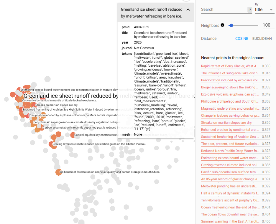
Using the UMAP algorithm for clustering (click ‘UMAP’ at the bottom left), we can now begin to explore the clusters. UMAP often has some points that I like to explore. Selecting one at random (‘Greenland ice sheet runoff reduced by meltwater refreezing…’), the projector highlights nearest neighbours and their similarity vectors.
In the top left, we can select to ‘color by’ the journal so that we can see the colors by journal. The broadest is ‘Nature Commun’ (i.e., Nature Communications), a broad, multi-disciplinary journal that covers a range of ideas.
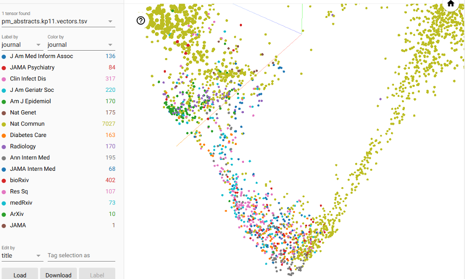
In contrast, there are a few tightly-clustered, like the American Journal of Epidemiology, Annals of Internal Medicine, Radiology, and Diabetes Care. Most of the other well-represented journals seem to overlap significantly.
Applications
What use is the tensor projector apart from presenting an attractive set of images? Fundamentally, I think it is most useful in helping to teach and comprehend what exactly embeddings are and how they work. In exploring these projections, it provides a spatial visualisation of an otherwise abstract idea (i.e., embedding vectors).
Additionally, the projector can be used to validate (or debug) generated embeddings to ensure they are behaving as expected: generating the appropriate relationships (or the lack thereof). Two models can even be projected and compared to help in selection or identifying problems.
There is also some code compiled to help with this process here: https://github.com/kpwhri/tensor_projector/.