
I’m quite accustomed to looking at performance against some gold (or silver) standard. It’s nice to have some ready definition of ‘truth’ and then, when applying some algorithm, we can clearly see if it matched or failed to match.
More recently, however, I was attempting to compare the outputs of multiple UMLS-processing NLP systems on a large dataset of notes. By default, these pieces of text are divided into multiple lines for storage (so that the database column can have fixed width). Merging these together can be somewhat complex for certain programming languages (e.g., SAS), so did we really need to do it? The analysis pitted cTAKES against MetaMap and MetaMapLite, using different underlying datasets and configurations. Each of these parameter sets was run against a corpus where the notes were reconstituted, and another one where they were not. If the performance was more or less equivalent, we could dispense with the costly process of joining all these lines.
The experiments were run, and the data extracted using the command line tools of mml_utils. Now, we end up with a dataframe for each experiment (e.g., NLP tool with parameter set), where each variables/columns represents a CUI, each record/row represents a unique note/document, and each value represents the count of that CUI in the note. We can concatenate these dataframes by moving the experiment to a separate variable/column.
| note_id | C0002792 | C0013404 | … | experiment |
| 0 | 1 | 4 | … | ctakes1 |
| 1 | 0 | 0 | … | ctakes1 |
| … | … | … | … | … |
| 0 | 0 | 3 | … | ctakes2 |
| 1 | 0 | 0 | … | ctakes2 |
Jaccard similarity does not care about the counts themselves, but only the presence/absence of a particular attribute. We will take the overlap (i.e., number of times the same CUI was found in the same note by both experiments) divided by the total number of CUIs which were found by either experiment (or both). We ignore when neither method found the CUI. Thus, in the table above, computing the Jaccard similarity for note_id #1, neither C0002791 nor C0013404 will contribute since they were not found.
| ctakes1 has count=0 | ctakes1 has count >= 1 | |
| ctakes2 has count=0 | Ignore | Denominator |
| ctakes2 has count >= 1 | Denominator | Numerator and Denominator |
For our little excerpt, the results would be the following for note_id #0:
| NOTE_ID = 0 | ctakes1 has count=0 | ctakes1 has count >= 1 |
| ctakes2 has count=0 | 0 | 1 |
| ctakes2 has count >= 1 | 0 | 1 |
Our Jaccard similarity for note_id #0 is: 1 / 1 + 0 + 1 or 0.5. For note_id #1, for our current excerpt, Jaccard similarity is undefined (i.e., there is nothing to compare).
This seemed easy to implement: we’re just calculating the intersection of CUIs divided by their union. Here’s my naive implementation:
dfs = []
experiments = list(df['experiment'].unique())
cuis = list(x for x in df.columns if x.startswith('C'))
docids = list(df.docid.unique())
for i, lexp in enumerate(experiments[:-1]):
    ldf = df[(df.experiment == lexp)][['docid'] + list(cuis)].set_index('docid').sort_index()
    for rexp in experiments[i + 1:]:
        name = f'{lexp}-{rexp}'
        rdf = df[(df.experiment == rexp)][['docid'] + list(cuis)].set_index('docid').sort_index()
        jaccard_coefs = []
        for docid in docids:
            # for each doc, get cuis where at least one appears in doc
            ls = ldf.T[docid]
            l_cuis = set(ls[ls > 0].index)
            rs = rdf.T[docid]
            r_cuis = set(rs[rs > 0].index)
            try:
                jac_coef = len(l_cuis & r_cuis) / len(l_cuis | r_cuis)
            except ZeroDivisionError:
                continue
            jaccard_coefs.append((docid, jac_coef, name))
        df_ = pd.DataFrame(jaccard_coefs, columns=['docid', 'jaccard', 'name'])
        dfs.append(df_)
jac_df = pd.concat(dfs)The constant indexing of dataframes with sorting is problematic, and the iteration through lots of dataframes seems less than ideal. It almost seems better if all of the notes and experiments were set as columns. This might be a more efficient approach?
Let’s reformat the dataframe:
df = df.set_index(['experiment', 'docid']).T| ctakes1 | ctakes1 | ctakes2 | ctakes2 | |
| cui \ note_id | 0 | 1 | 0 | 1 |
| C0002792 | 1 | 0 | 0 | 0 |
| C0013404 | 4 | 0 | 3 | 0 |
| … |
And our implementation with this quite wide dataframe:
dfs = []  # TODO: replace with `jaccard_coefs`
for i, lexp in enumerate(experiments[:-1]):
    for rexp in experiments[i + 1:]:
        name = f'{lexp}-{rexp}'
        jaccard_coefs = []  # TODO: this should be moved outside for loops
        for docid in docids:
            # for each doc, get cuis where at least one appears in doc
            ls = df[lexp][docid]
            l_cuis = set(ls[ls > 0].index)
            rs = df[rexp][docid]
            r_cuis = set(rs[rs > 0].index)
            try:
                jac_coef = len(l_cuis & r_cuis) / len(l_cuis | r_cuis)
            except ZeroDivisionError:
                continue
            jaccard_coefs.append((docid, jac_coef, name))
        df_ = pd.DataFrame(jaccard_coefs, columns=['docid', 'jaccard', 'name'])
        dfs.append(df_)
jac2_df = pd.concat(dfs) # TODO: just create dataframe once hereUnfortunately this takes 3 times as long (from 15 to 45 minutes).
Another similar approach will look to use a comparison of each column directly rather than using the union/intersection. We’ll also fix our loop to stop creating a bunch of unnecessary dataframes…and just simplify all the counts to 1.
df[df > 0] = 1

jaccard_coefs = []
for i, lexp in enumerate(experiments[:-1]):
    for rexp in experiments[i + 1:]:
        name = f'{lexp}-{rexp}'
        for docid in docids:
            # for each doc, get cuis where at least one appears in doc
            m01 = (df[lexp][docid].eq(0) & df[rexp][docid].eq(1)).sum()
            m10 = (df[lexp][docid].eq(1) & df[rexp][docid].eq(0)).sum()
            m11 = (df[lexp][docid].eq(1) & df[rexp][docid].eq(1)).sum()
            try:
                jac_coef = m11 / (m11 + m01 + m10)
            except ZeroDivisionError:
                continue
            jaccard_coefs.append((docid, jac_coef, name))
jac3_df = pd.DataFrame(jaccard_coefs, columns=['docid', 'jaccard', 'name'])This took even longer… I stopped it after an hour.
The inefficiencies here are likely due to having to approach multiple columns — what if all of the columns could just be compared against each other? Thus, instead of the index just being CUIs, it might be more efficient to have a multi-index of CUIs and the document.
First, we’ll place this into a long table format (via pd.melt):
| experiment | docid | cui | value |
| ctakes1 | 0 | C0002792 | 1 |
| ctakes1 | 0 | C0013404 | 1 |
| ctakes1 | 1 | C0002792 | 0 |
| ctakes1 | 1 | C0013404 | 0 |
| ctakes2 | 0 | C0002792 | 0 |
| ctakes2 | 0 | C0013404 | 1 |
| ctakes2 | 1 | C0002792 | 0 |
| ctakes2 | 1 | C0013404 | 0 |
df[df >= 1] = 1 has been applied.Next, we’ll pivot the table so that each column represents an experiment:
df = df.pivot(index=['docid', 'cui'], columns='experiment', values='value')| docid | cui | ctakes1 | ctakes2 | … |
| 0 | C0002792 | 1 | 0 | … |
| 0 | C0013404 | 1 | 1 | … |
| 1 | C0002792 | 0 | 0 | … |
| 1 | C0013404 | 0 | 0 | … |
| … | … | … | … | … |
Now, we can calculate the jaccard similarity for the entire experiment:
jaccard_coefs = []
for i, lexp in enumerate(experiments[:-1]):
    for rexp in experiments[i + 1:]:
        name = f'{lexp}-{rexp}'
        # for each doc, get cuis where at least one appears in doc
        m01 = (df[lexp].eq(0) & df[rexp].eq(1)).sum()
        m10 = (df[lexp].eq(1) & df[rexp].eq(0)).sum()
        m11 = (df[lexp].eq(1) & df[rexp].eq(1)).sum()
        try:
            jac_coef = m11 / (m11 + m01 + m10)
        except ZeroDivisionError:
            continue
        jaccard_coefs.append((jac_coef, name))
jac4_df = pd.DataFrame(jaccard_coefs, columns=['jaccard', 'name'])While this provides the similarity of the entire experiment, it doesn’t allow us to see how the similarity may vary across documents. With the first three methods (all produce an identical dataset), we can build a chart to visualise how the notes vary between methods.
Visualisation with seaborn
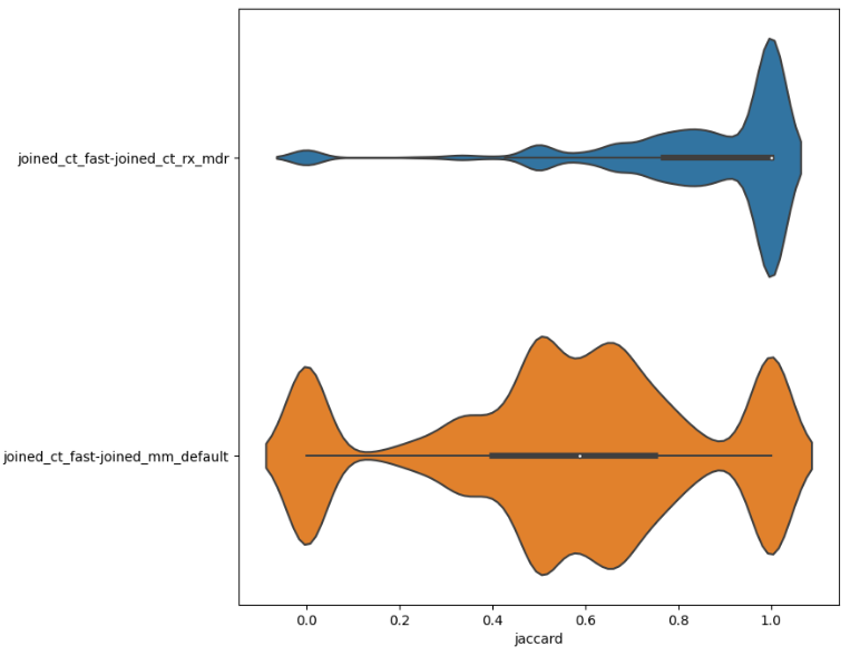
We can visualise the distribution of Jaccard similarity using seaborn.
import seaborn as sns


names = list(jac_df.name.unique())
plt.figure(figsize=(8, len(names))
ax = sns.violinplot(
    data=jac_df,
    y='name', x='jaccard', scale='width',
)This will, e.g., show us the close similarity between using the same NLP tool (ct=ctakes) under different settings vs. two separate NLP tools (mm=Metamap).
A heatmap can also be particularly instructive, showing at a glance how different methods compare. In the following, we will combine by finding the mean, but the median would also be instructive to explore.
# split name into left/right
jac_df['left'] = jac_df.name.str.split('-').str[0]
jac_df['right'] = jac_df.name.str.split('-').str[-1]
# find comparisons, but this is only the top right corner
c_df = jac_df.groupby(['left', 'right'])['jaccard'].mean().reset_index()
# create second dataframe, switch right/left labels
c2_df = c_df.copy()
c2_df.columns = ['right', 'left', 'jaccard']
# combine top left and bottom right halves together
hm_df = pd.concat((c_df, c2_df)).pivot(
    index='left', columns='right', values='jaccard'
).fillna(1)  # fill when comparing algorithm to itself
sns.heatmap(hm_df)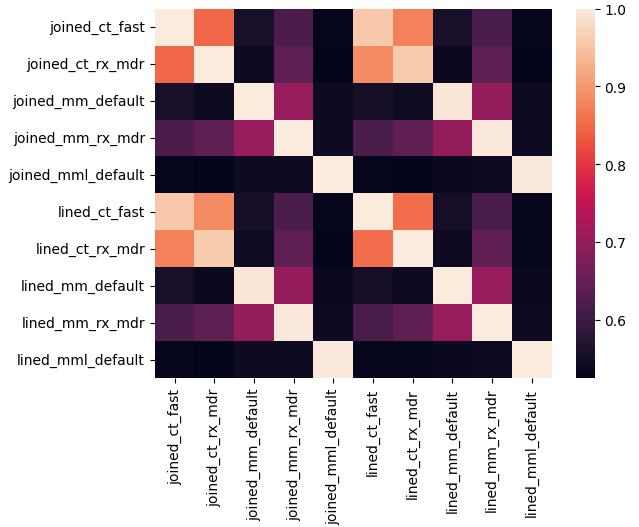
ct: ctakes, mm: metamap, mml: metamaplite.